Dynamic Mode Decomposition

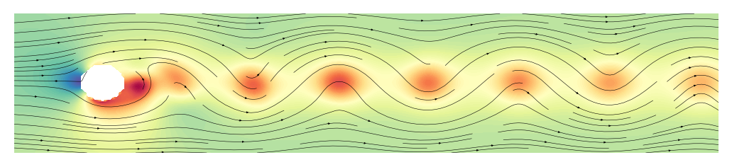
In this textbook example, we show how kooplearn can produce the dynamic mode decomposition of a fluid flow with very little effort. We will use data from FlowBench of a fluid flow past an object. First we download and display the data:

import os
import urllib.request

# Base URL for raw file downloads
base_url = "https://huggingface.co/datasets/BGLab/FlowBench/resolve/main/FPO_NS_2D_1024x256/harmonics/92/"

# List the exact filenames you want to download
filenames = [
    "input_geometry.npz",
    "Re_411.npz",  # Simulations at Reynolds number 411
]

print(f"Starting download from: {base_url}")

for fname in filenames:
    file_url = base_url + fname
    local_path = os.path.join(".", fname)  # Saves to the current directory

    # Check if the file already exists
    if os.path.exists(local_path):
        print(f"File already exists: {local_path}. Skipping.")
        continue  # Move to the next file

    # Proceed with download if it doesn't exist
    try:
        print(f"Downloading: {fname}...")
        # urlretrieve(source_url, destination_path)
        urllib.request.urlretrieve(file_url, local_path)
        print(f"Successfully saved to: {local_path}")
    except Exception as e:
        print(f"Failed to download {fname}: {e}")

print("All downloads finished.")

Starting download from: https://huggingface.co/datasets/BGLab/FlowBench/resolve/main/FPO_NS_2D_1024x256/harmonics/92/
File already exists: ./input_geometry.npz. Skipping.
File already exists: ./Re_411.npz. Skipping.
All downloads finished.

import matplotlib.pyplot as plt
import numpy as np

SUBSAMPLE = 4
flow = np.load("Re_411.npz")

X = flow["data"][:,::SUBSAMPLE, ::SUBSAMPLE, :]
geometry = np.load("input_geometry.npz")["mask"][::SUBSAMPLE, ::SUBSAMPLE]

def plot_flow(X, ax, time_id=0, streamplot: bool = True):
    u = X[..., 0]
    v = X[..., 1]
    p = X[..., 2]
    x, y = np.meshgrid(
        np.linspace(0, 5, 1024)[::SUBSAMPLE],
        np.linspace(0, 1, 256)[::SUBSAMPLE],
    )
    ax.set_aspect("equal")
    masked_pressure = np.where(
        geometry, p[time_id], np.nan
    )
    _ = ax.contourf(x, y, masked_pressure, 100, cmap="Spectral")
    if streamplot:
        ax.streamplot(
            x, y, u[time_id], v[time_id], color="black", linewidth=0.2, arrowsize=0.2
        )
    ax.set_axis_off()
    return ax

fig, ax = plt.subplots(dpi=200)
ax = plot_flow(X, ax)

Dynamic Mode Decomposition

kooplearn estimators have a convenient .dynamical_modes method which returns the Koopman mode decomposition. The original dynamic mode decomposition assumed a linear dynamics, and we will do the same in this notebook. First we properly scale and flatten the data using sklearn-compatible transformations:

from sklearn.base import BaseEstimator, TransformerMixin
from sklearn.pipeline import Pipeline

from kooplearn.preprocessing import FeatureFlattener

# Custom scaler. Can't use sklearn StandardScaler, as it improperly averages over every dimension,
# while we want to keep the field-wise means and stds separate.
class FlowScaler(BaseEstimator, TransformerMixin):
    def fit(self, X, y=None):
        # Save shape for inverse_transform
        self.mean_ = np.mean(X, axis =(0, 1, 2), keepdims=True)
        self.std_ = np.std(X, axis =(0, 1, 2), keepdims=True)
        self._is_fitted = True
        return self

    def transform(self, X, y=None):
        _X = (X - self.mean_)/self.std_
        return _X

    def inverse_transform(self, X, y=None):
        _X =  X*self.std_ + self.mean_
        return _X

flattener = FeatureFlattener()
scaler = FlowScaler()
data_pipe = Pipeline([("scaler", scaler),("flattener", flattener)])

We can now fit a kooplearn estimator. We will use the KernelRidge class, with a linear kernel. The results would be identical to using kooplearn.linear_model.Ridge, but the latter is better suited for large number of points and moderate number of dimentions.

from kooplearn.kernel import KernelRidge

model = KernelRidge(n_components=128, reduced_rank=False, alpha=1e-5)
model.fit(data_pipe.fit_transform(X))
# Compute the dynamical modes
dmd = model.dynamical_modes(data_pipe.fit_transform(X))

We can display a handy summary of the fitted model by calling the summary() method:

dmd.summary().head()

	frequency	lifetime	eigenvalue_real	eigenvalue_imag	eigenvalue_magnitude	is_stable	is_conjugate_pair
0	0.000000	4.016156e+08	1.000000	0.000000	1.000000	True	False
1	0.044882	2.836224e+04	0.960466	-0.278269	0.999965	True	True
2	0.056141	1.451679e+04	0.938365	-0.345448	0.999931	True	True
3	0.089713	9.749367e+03	0.845205	-0.534251	0.999897	True	True
4	0.033699	2.466430e+03	0.977271	-0.210071	0.999595	True	True

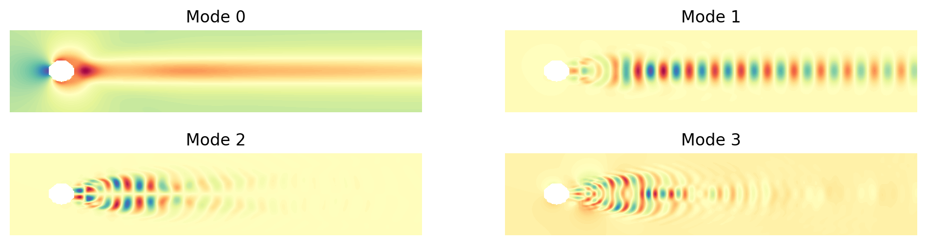
Finally, we can plot the leading modes:

# Some nice plots
import warnings

warnings.filterwarnings("ignore") # Suppress warning from annoying sklearn pipelines (see https://stackoverflow.com/questions/67943229/sklearn-pipeline-instance-is-not-fitted-yet-error-even-though-it-is)
t_id = 100
fig, axs = plt.subplots(ncols=2, nrows=2, figsize=(12, 3), dpi=200)
for mode_idx, ax in enumerate(axs.flatten()):
    ax = plot_flow(data_pipe.fit(X).inverse_transform(dmd[mode_idx]), ax = ax, streamplot=False)
    ax.set_title(f"Mode {mode_idx}")