Switching System

Author: Grégoire Pacreau, Pietro Novelli

In this example we show how kooplearn can be used to analyze the behaviour of a switching system, validating our results with Fourier theory. We study a simple signal composed by a sum of a small number of sinusoidal functions. These signals are easily analyzed using Fourier theory, but similar results can be obtained via Koopman theory and its implementation in kooplearn. In particular, we show that how to recover changes in the signal by detecting changes in the underlying process. Here, this will be modeled by a sudden change of the dominant frequencies of the signal during a switching period.

Data generation

In the following we define a function generating a purely oscillatory linear dynamical system with given frequencies.

import numpy as np
import scipy


def make_oscillatory_matrix(frequencies, dt=1.0):
    blocks = []
    for f in frequencies:
        if f < 0:
            raise ValueError("Frequencies must be non-negative.")
        omega = 2 * np.pi * f
        theta = omega * dt
        rotation_matrix = np.array(
            [[np.cos(theta), -np.sin(theta)], [np.sin(theta), np.cos(theta)]]
        )
        blocks.append(rotation_matrix)

    return scipy.linalg.block_diag(*blocks)

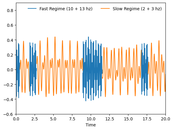
We can now create our signal. The signal in the first (fast) regime has frequencies 10Hz and 13Hz. The signal in the second (slow) regime has frequencies 2Hz and 3Hz.

from kooplearn.datasets import make_regime_switching_var

dt = 0.01
n_steps = 2000
noise = 0.001
fast_frequencies = [10, 13]
fast_phi = make_oscillatory_matrix(fast_frequencies, dt=dt)
slow_frequencies = [2, 3]
slow_phi = make_oscillatory_matrix(slow_frequencies, dt=dt)
regime_transition_matrix = np.array([[0.99, 0.01], [0.005, 0.995]])
# Initial state
X0 = 0.1 * np.ones(slow_phi.shape[0])

X = make_regime_switching_var(
    X0,
    fast_phi,
    slow_phi,
    regime_transition_matrix,
    n_steps=n_steps,
    noise=noise,
    dt=dt,
    random_state=0
)
y = X.values.sum(axis=1) # Sum the states into a single signal
times = X.index.get_level_values("time")
regimes = X.attrs['regimes']
fast_y = np.ma.masked_where(regimes == 1, y)
slow_y = np.ma.masked_where(regimes == 0, y)

Let’s plot the trajectories of our dataset

import matplotlib.pyplot as plt

fig, ax = plt.subplots()
ax.plot(times, fast_y, label="Fast Regime (10 + 13 hz)")
ax.plot(times, slow_y, label="Slow Regime (2 + 3 hz)")
ax.legend(frameon=False, ncols=2)
ax.set_xlabel("Time")
ax.set_ylim(-0.6, 0.9)
ax.margins(0)

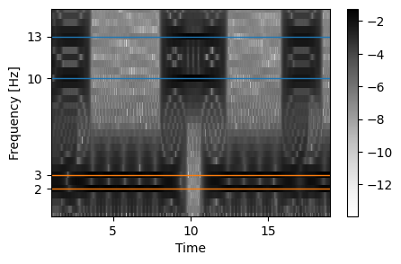
Let us verify that we do recover those frequencies using the classical Fourier spectrogram as implemented in scipy.signal.

from scipy import signal

n_seg = 200
res_spectrogram = signal.spectrogram(
    y, dt**-1, scaling="density", nperseg=n_seg, noverlap=n_seg - 1
)

fig, ax = plt.subplots(figsize=(5, 3))
pcolor = ax.pcolormesh(
    res_spectrogram[1], res_spectrogram[0], np.log10(res_spectrogram[2]), cmap="Greys"
)
ax.set_ylabel("Frequency [Hz]")
ax.set_xlabel("Time")
ax.set_yticks(fast_frequencies + slow_frequencies)
ax.set_ylim(0, 15)
for f in slow_frequencies:
    ax.axhline(y=f, color="tab:orange", lw=1)
for f in fast_frequencies:
    ax.axhline(y=f, color="tab:blue", lw=1)
fig.colorbar(pcolor)

<matplotlib.colorbar.Colorbar at 0x116af34d0>

Fitting the Kooplearn model

from kooplearn.kernel import KernelRidge
from kooplearn.preprocessing import TimeDelayEmbedding

We use a time delay embedding with 5 snapshots of history to fit the Koopman operator model.

td = TimeDelayEmbedding(history_length=5).fit(X)
model = KernelRidge(
    n_components=24, kernel="rbf", alpha=1e-6, gamma=0.1, eigen_solver="arpack"
).fit(td.transform(X))

dynamical_modes = model.dynamical_modes(td.transform(X))
dynamical_modes.summary(dt=dt).head(5)

	frequency	lifetime	eigenvalue_real	eigenvalue_imag	eigenvalue_magnitude	is_stable	is_conjugate_pair
0	0.000000	9132.375181	0.999999	0.000000	0.999999	True	False
1	3.014476	9.884760	0.981123	-0.188084	0.998989	True	True
2	2.013758	9.684646	0.990982	-0.126061	0.998968	True	True
3	12.947025	1.952708	0.683461	-0.722974	0.994892	True	True
4	9.960750	1.944084	0.806306	-0.582783	0.994869	True	True

Note that we have found modes around 13, 10, 3, and 2 Hz, as expected. The slow modes (low frequency) have a longer lifetime than the fast frequency ones, as expected. Indeed, the switching from slow to fast regime is governed by a geometric distribution with parameter \(p\) given by regime_transition_matrix[1, 0] = 0.005 while switching from fast to slow will be regime_transition_matrix[0, 1] = 0.01.

fig, axs = plt.subplots(ncols=2, figsize=(12, 3))
# We invert the time delay embedding to have the dynamical modes only for the true dynamical state.
slow_modes = (td.inverse_transform(dynamical_modes[1]) +
              td.inverse_transform(dynamical_modes[2])).sum(axis=-1)
fast_modes = (td.inverse_transform(dynamical_modes[3]) +
              td.inverse_transform(dynamical_modes[4])).sum(axis=-1)
axs[0].plot(times, y, color="k", lw=0.5, alpha=0.4)
axs[0].plot(times, slow_modes, color="tab:orange")
axs[0].set_title("Slow Modes")
axs[0].set_xlabel("Time")

axs[1].plot(times, y, color="k", lw=0.5, alpha=0.4)
axs[1].plot(times, fast_modes, color="tab:blue")
axs[1].set_title("Fast Modes")
axs[1].set_xlabel("Time")

Text(0.5, 0, 'Time')

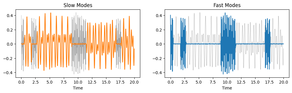
As we can see, the dynamical models associated to the low frequencies perfectly capture the “slow regime”, and vanish in the fast regime. Similarly, the high-frequency modes lights up in the fast regime, and are none elsewhere. Koopman dynamical modes, therefore, automatically identify the different regimes and can be leveraged — for example taking their expected value over short time windows — to detect regime switching.