Estimating Eigenfunctions of the Transfer Operator

Author: Pietro Novelli

This example is a reproduction of the second experiment of “Sharp Spectral Rates for Koopman Operator Learning”[1]. We use kooplearn to approximate the leading eigenfunctions of the transfer operator of the overdamped Langevin dynamics

\[X_{t + 1} = X_t -\frac{1}{\gamma}\nabla V(X_t)\Delta t + \frac{\sigma}{\gamma}\sqrt{\Delta t}\xi_t\]

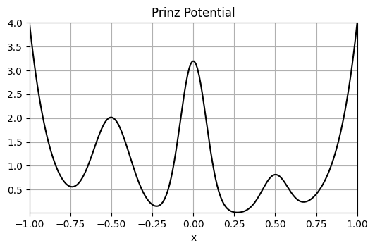
Here, \(V\) is the potential function, \(\gamma\) is a damping coefficient, and \(\sigma\) is proportional to the temperature of the process: the higher the \(\sigma\), the noisier is the dynamics. In this example we will study the so-called Prinz Potential[2]:

import matplotlib.pyplot as plt
import numpy as np

plt.rcParams["figure.figsize"] = [6.0, 3.5]


def prinz_potential(x):
    return 4 * (
        x**8
        + 0.8 * np.exp(-80 * (x**2))
        + 0.2 * np.exp(-80 * ((x - 0.5) ** 2))
        + 0.5 * np.exp(-40 * ((x + 0.5) ** 2))
    )


x = np.linspace(-1, 1, 200)
plt.plot(x, prinz_potential(x), "k")
plt.margins(0)
plt.xlabel("x")
plt.title("Prinz Potential")
plt.grid()

kooplearn exposes the function make_prinz_potential to simulate the overdamped Langevin dynamics with this potential.

from kooplearn.datasets import make_prinz_potential

gamma = 1.0
sigma = 2.0
data = make_prinz_potential(X0=0, n_steps=int(5e6), gamma=gamma, sigma=sigma)

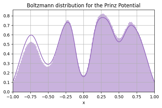
for overdamped Langevin processes, the inverse temperature satisfies the relation \(\beta = 2\gamma/\sigma^2\). With this, we can easily verify that data approximately samples the Boltzmann distribution \(e^{-\beta V(x)}\).

from scipy.integrate import romb


def compute_boltzmann_density(x, gamma, sigma):
    beta = 2 * gamma / (sigma**2)
    pdf = np.exp(-beta * prinz_potential(x))
    total_mass = romb(pdf, dx=x[1] - x[0])
    return pdf / total_mass


x = np.linspace(-2, 2, 2048 + 1)
density = compute_boltzmann_density(x, gamma, sigma)
plt.hist(data, bins=200, density=True, alpha=0.5, color="tab:purple")
plt.plot(x, density, color="tab:purple")
plt.xlim(-1, 1)
plt.grid()
plt.title("Boltzmann distribution for the Prinz Potential")
plt.xlabel("x")

Text(0.5, 0, 'x')

Estimating the eigenfunctions

We will compare the Reduced Rank Regression estimator [3] against the classical Principal Component estimator, also known as kernel DMD [4]. To this end, we use kooplearn’s KernelRidge class, with a simple Gaussian kernel (rbf).

from kooplearn.kernel import KernelRidge

n_train_samples = 5001


def fit_and_estimate(reduced_rank, x, density, random_state):
    subsample = 100  # We need long trajectories to sample the Boltzmann distribution...
    gamma = 1.0
    sigma = 2.0
    data = make_prinz_potential(
        X0=0, n_steps=int(7e5), gamma=gamma, sigma=sigma, random_state=random_state
    )
    data = data.iloc[
        ::subsample
    ]  # ...but we don't need all the data to estimate the eigenfunctions
    data = data[:n_train_samples]
    model = KernelRidge(
        n_components=5,
        reduced_rank=reduced_rank,
        gamma=12.5,
        kernel="rbf",
        alpha=1e-6,
        random_state=random_state,
    )  # Model definition
    model.fit(data)
    values, functions = model.eig(eval_right_on=x)  # Eigenvalue estimation
    sort_perm = np.flip(np.argsort(np.abs(values)))  # Order eigenvalues decreasingly
    values, functions = values[sort_perm], functions[:, sort_perm]
    functions = normalize_eigenfunctions(functions, x, density)
    return functions


def normalize_eigenfunctions(functions, x, density):
    abs2_eigfun = (np.abs(functions) ** 2).T  # f(x)**2
    abs2_eigfun *= density  # Compute the norm with respect to the Boltzmann measure.
    dx = x[1] - x[0]
    funcs_norm = np.sqrt(romb(abs2_eigfun, dx=dx, axis=1))  # Norms
    functions *= funcs_norm**-1.0  # Normalize
    return functions

The code above is straightforward: the function fit_and_estimate samples a fresh new trajectory, fits a transfer operator model, computes its (right) eigenfunctions via model.eig, and evaluates it on the array x via the argument eval_right_on=x. Finally, it computes the normalization constant

\[\left(\int e^{-\beta V(x)} |\psi(x)|^2dx\right)^{1/2}\]

via the normalize_eigenfunctions helper method. We now run this function for both Reduced Rank (reduced_rank = True) and Principal Component (reduced_rank = False) estimators. To gather some statistics, we repeat the evaluation multiple times.

from collections import defaultdict

from tqdm import tqdm

dt = 1e-4
n_repetitions = 10
results = defaultdict(list)
for method, reduced_rank in zip(
    ["Principal Components (kDMD)", "Reduced Rank"], [False, True]
):
    for i in tqdm(range(n_repetitions)):
        results[method].append(fit_and_estimate(reduced_rank, x[:, None], density, i))

100%|██████████| 10/10 [00:22<00:00,  2.30s/it]
100%|██████████| 10/10 [00:48<00:00,  4.86s/it]

let’s print some results

fig, axs = plt.subplots(ncols=4, figsize=(9, 2))
for fun_id, ax in enumerate(axs):
    for method, functions in results.items():
        color = "tab:blue" if "Principal" in method else "tab:orange"
        ax.plot(x, functions[0][:, fun_id], color=color, label=method)
    ax.set_title(rf"Eigenfunction $\psi_{fun_id}$", fontsize=9)
    ax.set_xlim(-1, 1)
handles, labels = ax.get_legend_handles_labels()
fig.legend(
    handles,
    labels,
    loc="upper center",
    ncols=2,
    frameon=False,
    bbox_to_anchor=(0.0, 1.05, 1.0, 0.102),
)

<matplotlib.legend.Legend at 0x11efbe490>

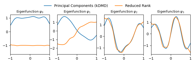
As we can see, some eigenfunctions seem to have a sign mismatch. This is to be expected, as the spectral decomposition is not unique, and multiplying by a constant scalar value (including -1), returns a valid eigenvector. To overcome this issue, we can write down a simple helper function to standardize them

def standardize_sign(eigenfunction, reference, x):
    eigenfunction_cut = cut_functions_to_domain(eigenfunction, x)
    reference_cut = cut_functions_to_domain(reference, x)
    norm_p = np.linalg.norm(eigenfunction_cut + reference_cut)
    norm_m = np.linalg.norm(eigenfunction_cut - reference_cut)
    if norm_p <= norm_m:
        return -1.0 * eigenfunction
    else:
        return eigenfunction


def cut_functions_to_domain(functions, x, x_lims=(-1, 1)):
    mask = (x >= x_lims[0]) & (x <= x_lims[1])
    return functions[mask]


def compute_ylims(reference, margin=0.1):
    ref_min = reference.min()
    ref_max = reference.max()
    if ref_min < 0:
        ref_min *= 1 + margin
    else:
        ref_min *= 1 - margin
    if ref_max < 0:
        ref_max *= 1 - margin
    else:
        ref_max *= 1 + margin

    y_min = np.round(ref_min, 1)
    y_max = np.round(ref_max, 1)
    return y_min, y_max

kooplearn also exposes the function compute_prinz_potential_eig returning the exact eigenfunctions associated to the Prinz Potential dynamics. We will now use it to get the reference eigenfunctions, so that we can compare our estimators:

from kooplearn.datasets import compute_prinz_potential_eig

dt = data.attrs["params"]["dt"]
_, reference_eigfuns = compute_prinz_potential_eig(
    gamma, sigma, dt, eval_right_on=x, num_components=5
)
reference_eigfuns = normalize_eigenfunctions(reference_eigfuns, x, density)

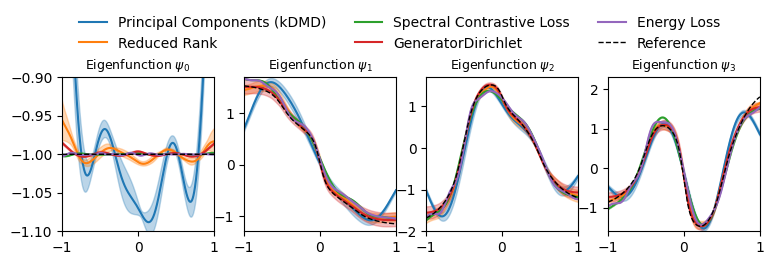
we can finally plot everything together

def plot_eigenfunctions_with_uncertainty(results, reference_eigfuns, x):
    tab_colors = plt.get_cmap("tab10").colors
    fig, axs = plt.subplots(ncols=4, figsize=(9, 2))
    for fun_id, ax in enumerate(axs):
        reference = reference_eigfuns[:, fun_id]
        for color, (method, functions) in zip(tab_colors, results.items()):
            # Standardize signs according to the reference
            functions = np.array(functions)  # Convert list of arrays into array
            n_repetitions = functions.shape[0]
            for i in range(n_repetitions):
                for j in range(4):
                    functions[i, :, j] = standardize_sign(
                        functions[i, :, j], reference_eigfuns[:, j], x
                    )
            m = functions.mean(0)[:, fun_id].real
            st = functions.std(0)[:, fun_id].real
            ax.plot(x, m, color=color, label=method)
            ax.fill_between(x, m - st, m + st, color=color, alpha=0.3)
            ax.set_ylim(compute_ylims(reference))
        ax.plot(x, reference, color="k", lw=1, ls="--", label="Reference")
        ax.set_title(rf"Eigenfunction $\psi_{fun_id}$", fontsize=9)
        ax.set_xlim(-1, 1)
    handles, labels = ax.get_legend_handles_labels()
    ncols = 2 if (len(results) + 1) == 4 else 3
    fig.legend(
        handles,
        labels,
        loc="upper center",
        ncols=ncols,
        frameon=False,
        bbox_to_anchor=(0.0, 1.15, 1.0, 0.102),
    )


plot_eigenfunctions_with_uncertainty(results, reference_eigfuns, x)

…showing that the Reduced Rank estimator approximates the reference eigenfunctions much better than the more common Principal Component Regression (kernel DMD).

A Representation Learning Approach

We now move beyond classical kernel methods by exploring a representation learning approach. We aim to learn a mapping \(\varphi\) that transforms the system’s state into a latent space where the evolution of dynamics is linear, effectively approximating the eigenfunctions.

Spectral Contrastive Loss

To achieve this, we train an encoder-only model optimized via the SpectralContrastiveLoss.

The model architecture is twofold:

• Encoder: A Multilayer Perceptron (MLP) that lifts the state to the latent space.

• Predictor: A linear layer that evolves the state forward in time.

See “Self-Supervised Evolution Operator Learning for High-Dimensional Dynamical Systems” [5] for the theoretical background.

import torch

n_train_samples = 5000
n_val_samples = 1000

subsample = 100
data = make_prinz_potential(
    X0=0, n_steps=int(7e5), gamma=gamma, sigma=sigma, random_state=0
)
data = data.iloc[
    ::subsample
]  # ...but we don't need all the data to estimate the eigenfunctions

train_data = torch.from_numpy(data[:n_train_samples].values).float()
val_data = torch.from_numpy(data[-n_val_samples:].values).float()

We now implement the training script for the spectral contrastive loss:

from torch.utils.data import DataLoader, TensorDataset

batch_size = 512

# Creating PyTorch TensorDatasets
train_ds = TensorDataset(train_data[:-1], train_data[1:])
val_ds = TensorDataset(val_data[:-1], val_data[1:])

# Creating DataLoaders
train_dl = DataLoader(train_ds, batch_size=batch_size, shuffle=True)
val_dl = DataLoader(val_ds, batch_size=len(val_ds), shuffle=False)

# Experiment hyperparameters
learning_rate = 1e-2
opt = torch.optim.AdamW
num_epochs = 200
layer_dims = [32, 64, 32]
latent_dim = 32
random_state = 42

class SimpleMLP(torch.nn.Module):
    def __init__(
        self, latent_dim: int, layer_dims: list[int], activation=torch.nn.SiLU
    ):
        super().__init__()
        self.activation = activation
        lin_dims = [1] + layer_dims + [latent_dim]

        layers = []

        for layer_idx in range(len(lin_dims) - 2):
            layers.append(
                torch.nn.Linear(
                    lin_dims[layer_idx], lin_dims[layer_idx + 1], bias=False
                )
            )
            layers.append(activation())

        layers.append(torch.nn.Linear(lin_dims[-2], lin_dims[-1], bias=True))

        self.layers = torch.nn.ModuleList(layers)

    def forward(self, x):
        # MLP
        for layer in self.layers:
            x = layer(x)
        return x

from kooplearn.linear_model import Ridge
from kooplearn.torch.utils import FeatureMapEmbedder

device = "cuda" if torch.cuda.is_available() else "cpu"


class FeatureMap(torch.nn.Module):
    def __init__(self, latent_dim: int, normalize_latents: bool = False):
        super().__init__()
        self.normalize_latents = normalize_latents
        self.backbone = SimpleMLP(latent_dim=latent_dim, layer_dims=layer_dims)
        self.lin = torch.nn.Linear(latent_dim, latent_dim, bias=False)

    def forward(self, X, lagged: bool = False):
        z = self.backbone(X)
        if self.normalize_latents:
            z = torch.nn.functional.normalize(z, dim=-1)
        if lagged:
            z = self.lin(z)
        return z


def train_encoder_only(criterion: torch.nn.Module):
    torch.manual_seed(random_state)
    # Initialize model, loss and optimizer
    model = FeatureMap(latent_dim).to(device)
    optimizer = opt(model.parameters(), lr=learning_rate)

    def step(batch, is_train: bool = True):
        batch_X, batch_Y = batch
        batch_X, batch_Y = batch_X.to(device), batch_Y.to(device)
        if is_train:
            optimizer.zero_grad()
        phi_X, phi_Y = model(batch_X), model(batch_Y, lagged=True)
        loss = criterion(phi_X, phi_Y)
        if is_train:
            loss.backward()
            optimizer.step()
        return loss.item()

    for epoch in range(num_epochs):
        # Training phase
        model.train()
        train_loss = []
        for batch in train_dl:
            train_loss.append(step(batch))
        # Validation phase
        model.eval()
        val_loss = []
        with torch.no_grad():
            for batch in val_dl:
                val_loss.append(step(batch, is_train=False))

        if (epoch + 1) % 10 == 0 or (epoch == 0):
            print(
                f"EPOCH {epoch + 1:>2}  Loss: {np.mean(train_loss):.2f} (train) -  " /
                f"{np.mean(val_loss):.2f} (val)"
            )

    embedder = FeatureMapEmbedder(encoder=model, device=device)
    evolution_operator_model = Ridge(n_components=latent_dim).fit(
        embedder.transform(train_data), train_data.numpy(force=True)
    )

    return {
        "model": evolution_operator_model,
        "feature_map": embedder.transform,
    }

from kooplearn.torch.nn import SpectralContrastiveLoss

trained_models = {}
trained_models["Spectral Contrastive Loss"] = train_encoder_only(
    SpectralContrastiveLoss()
)

EPOCH  1  Loss: -0.85 (train) -  -1.81 (val)
EPOCH 10  Loss: -2.01 (train) -  -2.17 (val)
EPOCH 20  Loss: -2.51 (train) -  -2.44 (val)
EPOCH 30  Loss: -2.55 (train) -  -2.55 (val)
EPOCH 40  Loss: -2.96 (train) -  -2.93 (val)
EPOCH 50  Loss: -3.01 (train) -  -2.96 (val)
EPOCH 60  Loss: -2.99 (train) -  -2.89 (val)
EPOCH 70  Loss: -3.06 (train) -  -3.00 (val)
EPOCH 80  Loss: -3.08 (train) -  -3.02 (val)
EPOCH 90  Loss: -3.08 (train) -  -3.00 (val)
EPOCH 100  Loss: -3.04 (train) -  -2.99 (val)
EPOCH 110  Loss: -3.11 (train) -  -2.96 (val)
EPOCH 120  Loss: -3.10 (train) -  -2.96 (val)
EPOCH 130  Loss: -3.17 (train) -  -3.02 (val)
EPOCH 140  Loss: -3.16 (train) -  -3.05 (val)
EPOCH 150  Loss: -3.17 (train) -  -3.03 (val)
EPOCH 160  Loss: -3.16 (train) -  -3.06 (val)
EPOCH 170  Loss: -3.17 (train) -  -3.09 (val)
EPOCH 180  Loss: -3.18 (train) -  -3.07 (val)
EPOCH 190  Loss: -3.19 (train) -  -3.10 (val)

Warning: The fitting algorithm discarded 14 dimensions of the 32 requested out of numerical instabilities.
The rank attribute has been updated to 18.
Consider decreasing the rank parameter.

EPOCH 200  Loss: -3.16 (train) -  -3.03 (val)

Now that the represntation has been learned, we compare the eigenfunctions to the reference as before

def estimate_representations(model, embedder, x, density):
    values, functions = model.eig(eval_right_on=embedder(x))  # Eigenvalue estimation
    sort_perm = np.flip(np.argsort(np.abs(values)))  # Order eigenvalues decreasingly
    values, functions = values[sort_perm], functions[:, sort_perm]
    functions = normalize_eigenfunctions(functions, x, density)
    return functions


for model_id, trained_model in trained_models.items():
    results[model_id] = [
        estimate_representations(
            trained_model["model"], trained_model["feature_map"], x[:, None], density
        )
    ]

plot_eigenfunctions_with_uncertainty(results, reference_eigfuns, x)

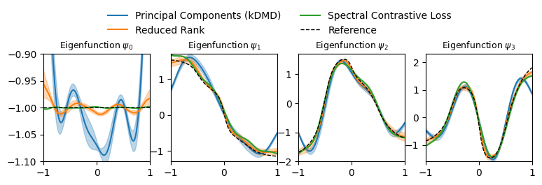
Notably, optimizing the mapping \(\varphi\) with the SpectralContrastiveLoss enables a precise estimation of eigenfunctions—including the trivial constant function \(\Psi_0\), which remains flat unlike in standard Reduced Rank models.

Generator learning

Similarly to the transfer operator approach, we now present two different estimators for learning the infinitesimal generator of the process. The first one uses kernel methods, while a second one leverages neural networks and representation learning.

In this section, we study the infinitesimal generator of a stochastic process, focusing on overdamped Langevin dynamics. The infinitesimal generator encodes the evolution of observables and plays a key role in analyzing long-time dynamics, metastable states, and spectral properties of the system.

The infinitesimal Generator

The infinitesimal generator \(\mathcal{L}\) describes the instantaneous evolution of smooth functions \(f: \mathbb{R}^d \to \mathbb{R}\) under the stochastic dynamics:

\[\mathcal{L} f(x) = \lim_{\Delta t \to 0} \frac{\mathbb{E}[f(X_{t + \Delta t}) \mid X_t = x] - f(x)}{\Delta t}.\]

For the overdamped Langevin process, the generator takes the form:

\[\mathcal{L} f(x) = - \frac{1}{\gamma} \nabla V(x) \cdot \nabla f(x) + \frac{\beta}{\gamma} \Delta f(x),\]

where (\(\Delta f = \nabla \cdot \nabla f\)) is the Laplacian.

Link with the transfer operator

The infinitesimal generator governs the evolution of observables under the stochastic dynamics, we define

\[u(x,t) = \mathbb{E}[f(X_t) \mid X_0 = x].\]

It satisfies the backward Kolmogorov equation:

\[\frac{\partial u}{\partial t}(x,t) = \mathcal{L} u(x,t), \quad u(x,0) = f(x).\]

From the perspective of transfer operators, the infinitesimal generator is the derivative of the Koopman operator at (t = 0):

\[\mathcal{L} f = \lim_{t \to 0} \frac{\mathcal{K}^t f - f}{t}.\]

Thus, \(\mathcal{L}\) can be viewed as the infinitesimal generator of the semigroup (\({\mathcal{K}^t}_{t \ge 0}\)).

Eigenfunctions of \(\mathcal{L}\) correspond to directions in function space that evolve exponentially under the Koopman operator:

\[\mathcal{K}^t \phi = e^{\lambda t} \phi, \quad \mathcal{L} \phi = \lambda \phi.\]

This perspective makes the connection between generator-based approaches and data-driven Koopman analysis explicit:

learning \(\mathcal{L}\) from data allows us to approximate the long-time dynamics, metastable states, and slow collective modes of the system.

Kernel methods

In this part we implement the method published in (Kostic et al 2024) based on the revolvent operator $ (\mu `I - :nbsphinx-math:mathcal{L}`)^{-1} $

from kooplearn.kernel._generator import GeneratorDirichlet


def fit_and_estimate_generator(x, density):
    subsample = 100  # We need long trajectories to sample the Boltzmann distribution...
    gamma = 1.0
    sigma = 2.0
    data = make_prinz_potential(X0=0, n_steps=int(5e5), gamma=gamma, sigma=sigma)
    data = data.values[
        ::subsample
    ]  # ...but we don't need all the data to estimate the eigenfunctions
    model = GeneratorDirichlet(
        diffusion=sigma / gamma, n_components=5, gamma=50, alpha=1e-5, shift=5
    )  # Model definition
    model.fit(data)
    values, functions = model.eig(eval_right_on=x)  # Eigenvalue estimation
    values, functions = values, functions
    functions = normalize_eigenfunctions(functions, x, density)
    return functions

results["GeneratorDirichlet"] = []
for _ in tqdm(range(n_repetitions)):
    results["GeneratorDirichlet"].append(
        fit_and_estimate_generator(x[:, None], density)
    )

100%|██████████| 10/10 [07:25<00:00, 44.51s/it]

plot_eigenfunctions_with_uncertainty(results, reference_eigfuns, x)

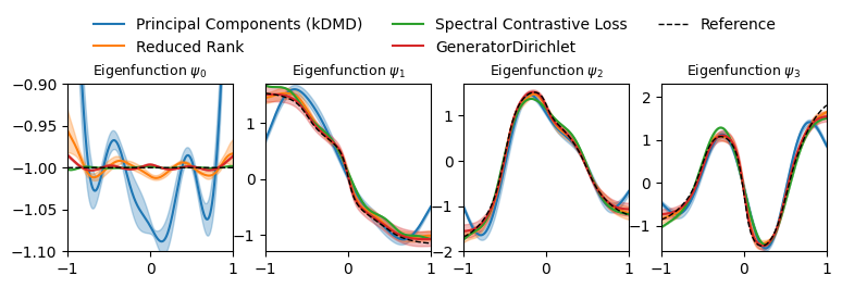
Energy Loss

The last method we explore still targets the infinitesimal generator of the process, but in contrast to GeneratorDirichlet it learns an appropriate representation, rather than using a prescribed kernel function. The fitting process is analogous the the spectral contrastive loss showed above.

from torch.utils.data import DataLoader, TensorDataset

batch_size = 512

# Creating PyTorch TensorDatasets
train_ds = TensorDataset(train_data[:-1])
val_ds = TensorDataset(val_data[:-1])

# Creating DataLoaders
train_dl = DataLoader(train_ds, batch_size=batch_size, shuffle=True)
val_dl = DataLoader(val_ds, batch_size=len(val_ds), shuffle=False)

from torch.func import functional_call, jacrev, vmap


class GeneratorFeatureMap(torch.nn.Module):
    def __init__(
        self, latent_dim: int, layer_dims: list[int], normalize_latents: bool = False
    ):
        super().__init__()
        self.normalize_latents = normalize_latents
        self.backbone = SimpleMLP(latent_dim=latent_dim, layer_dims=layer_dims)

    def compute_jacobian(self, x):
        """
        Efficiently computes the Jacobian of the output embeddings w.r.t the input x.

        This method uses `torch.func.vmap` and `torch.func.jacrev` to compute
        gradients. This is significantly faster than loop-based approaches and
        more memory-efficient than `torch.autograd.functional.jacobian` for batches.

        Parameters
        ----------
        x : torch.Tensor
            Input data of shape (batch_size, latent_dim).

        Returns
        -------
        torch.Tensor
            Jacobian tensor of shape (batch_size, latent_dim, output_dim).

            The element at index [b, i, j] corresponds to the partial derivative:
            $\\frac{\\partial \\text{output}[b, j]}{\\partial \\text{input}[b, i]}$
        """

        # Define a functional version of the forward pass for a single sample
        def func_forward(x_sample, params_buffers):
            out = functional_call(self.backbone, params_buffers, (x_sample,))
            if self.normalize_latents:
                out = torch.nn.functional.normalize(out, dim=-1)
            return out

        # Extract parameters/buffers (needed for functional_call)
        params = dict(self.backbone.named_parameters())
        buffers = dict(self.backbone.named_buffers())
        params_buffers = {**params, **buffers}

        # Compose vmap and jacrev
        # jacrev computes Jacobian of func_forward w.r.t arg 0 (x_sample)
        # vmap vectorizes this operation over the batch dimension (dim 0)
        compute_batch_jacobian = vmap(
            jacrev(func_forward, argnums=0), in_dims=(0, None)
        )

        # Execute
        jacobian = compute_batch_jacobian(x, params_buffers)

        # jacrev returns (output_dim, input_dim).
        # Since we are mapping R^d -> R^l, jacrev gives dU/dx.
        # Check shapes: resulting shape from vmap is (batch, output_dim, input_dim)
        # You wanted (batch, input_dim, output_dim), so we transpose.
        return jacobian.permute(0, 2, 1)

    def forward(self, x, return_grad: bool = False):
        # Standard forward pass
        z = self.backbone(x)
        if self.normalize_latents:
            z = torch.nn.functional.normalize(z, dim=-1)

        if return_grad:
            jacobian = self.compute_jacobian(x)
            return z, jacobian
        return z


def train_encoder_only(criterion: torch.nn.Module):
    torch.manual_seed(random_state)
    # Initialize model, loss and optimizer
    model = GeneratorFeatureMap(latent_dim, layer_dims).to(device)
    optimizer = opt(model.parameters(), lr=learning_rate)

    def step(batch, is_train: bool = True):
        X = batch[0]
        X = X.to(device)
        if is_train:
            optimizer.zero_grad()
        phi_X, grad_phi_X = model(X, return_grad=True)
        loss = criterion(phi_X, grad_phi_X)
        if is_train:
            loss.backward()
            optimizer.step()
        return loss.item()

    for epoch in range(num_epochs):
        # Training phase
        model.train()
        train_loss = []
        for batch in train_dl:
            train_loss.append(step(batch))
        # Validation phase
        model.eval()
        val_loss = []
        for batch in val_dl:
            val_loss.append(step(batch, is_train=False))

        if (epoch + 1) % 10 == 0 or (epoch == 0):
            print(
                f"EPOCH {epoch + 1:>2}  Loss: {np.mean(train_loss):.2f} (train) - " /
                f"{np.mean(val_loss):.2f} (val)"
            )

    embedder = FeatureMapEmbedder(encoder=model, device=device)
    evolution_operator_model = Ridge(n_components=latent_dim).fit(
        embedder.transform(train_data), train_data.numpy(force=True)
    )

    return {
        "model": evolution_operator_model,
        "feature_map": embedder.transform,
    }

from kooplearn.torch.nn import EnergyLoss

trained_models["Energy Loss"] = train_encoder_only(EnergyLoss(grad_weight=1e-3))

EPOCH  1  Loss: -1.26 (train) -  -1.83 (val)
EPOCH 10  Loss: -2.89 (train) -  -2.80 (val)
EPOCH 20  Loss: -2.94 (train) -  -2.95 (val)
EPOCH 30  Loss: -3.82 (train) -  -3.76 (val)
EPOCH 40  Loss: -4.65 (train) -  -4.56 (val)
EPOCH 50  Loss: -5.39 (train) -  -5.33 (val)
EPOCH 60  Loss: -5.59 (train) -  -5.52 (val)
EPOCH 70  Loss: -6.47 (train) -  -6.50 (val)
EPOCH 80  Loss: -7.04 (train) -  -6.87 (val)
EPOCH 90  Loss: -7.10 (train) -  -6.36 (val)
EPOCH 100  Loss: -7.19 (train) -  -7.04 (val)
EPOCH 110  Loss: -7.29 (train) -  -7.17 (val)
EPOCH 120  Loss: -7.53 (train) -  -7.46 (val)
EPOCH 130  Loss: -8.26 (train) -  -8.16 (val)
EPOCH 140  Loss: -8.32 (train) -  -8.34 (val)
EPOCH 150  Loss: -8.68 (train) -  -8.50 (val)
EPOCH 160  Loss: -8.58 (train) -  -8.28 (val)
EPOCH 170  Loss: -8.88 (train) -  -8.87 (val)
EPOCH 180  Loss: -9.25 (train) -  -9.10 (val)
EPOCH 190  Loss: -9.25 (train) -  -9.22 (val)

Warning: The fitting algorithm discarded 11 dimensions of the 32 requested out of numerical instabilities.
The rank attribute has been updated to 21.
Consider decreasing the rank parameter.

EPOCH 200  Loss: -9.28 (train) -  -9.37 (val)

results["Energy Loss"] = [
    estimate_representations(
        trained_models["Energy Loss"]["model"],
        trained_models["Energy Loss"]["feature_map"],
        x[:, None],
        density,
    )
]

plot_eigenfunctions_with_uncertainty(results, reference_eigfuns, x)

[1]

Vladimir R Kostic, Karim Lounici, Pietro Novelli, and Massimiliano Pontil. Sharp spectral rates for koopman operator learning. In Thirty-seventh Conference on Neural Information Processing Systems. 2023. URL: https://openreview.net/forum?id=Lt3jqxsbVO.

[2]

Jan-Hendrik Prinz, Hao Wu, Marco Sarich, Bettina Keller, Martin Senne, Martin Held, John D. Chodera, Christof Schütte, and Frank Noé. Markov models of molecular kinetics: generation and validation. The Journal of Chemical Physics, May 2011. URL: http://dx.doi.org/10.1063/1.3565032, doi:10.1063/1.3565032.

[3]

Vladimir Kostic, Pietro Novelli, Andreas Maurer, Carlo Ciliberto, Lorenzo Rosasco, and Massimiliano Pontil. Learning dynamical systems via koopman operator regression in reproducing kernel hilbert spaces. Advances in Neural Information Processing Systems, 35:4017–4031, 2022.

[4]

Matthew O. Williams, Clarence W. Rowley, and Ioannis G. Kevrekidis. A kernel-based method for data-driven koopman spectral analysis. Journal of Computational Dynamics, 2(2):247–265, 2015. URL: http://dx.doi.org/10.3934/jcd.2015005, doi:10.3934/jcd.2015005.

[5]

Giacomo Turri, Luigi Bonati, Kai Zhu, Massimiliano Pontil, and Pietro Novelli. Self-supervised evolution operator learning for high-dimensional dynamical systems. arXiv preprint arXiv:2505.18671, 2025.